Independent computational research
When Is a Two-State Tunneling Model Reliable?
Formal title · Testing the Validity of a Two-State Approximation in Double-Well Quantum Tunneling
How accurately can an effective two-state model reproduce right-well dynamics across a controlled double-well parameter grid, and which approximation layer limits that accuracy?
These counts describe whether each comparison can be evaluated reliably; they do not classify the two-state model as physically valid or invalid. The reliability masks are metric-specific: all 63 cases support RMSE comparisons, 52 also support maximum-error and strict full-dynamics extrema, and the remaining 11 still support RMSE, peak-time, and spectral analysis.
Key takeaway
Reliability depends on the question being asked.
This study compares an effective two-state model with a finite-difference, multi-eigenstate reference across a 63-case barrier-and-width grid.
All 63 cases support RMSE comparisons, while 52 support stricter maximum-error and full-dynamics extrema; the other 11 remain unresolved only for that stricter numerical analysis.
No final physical-validity threshold or universal failure boundary has been chosen.
01 / Research question
Why approximation validity matters.
Approximations make quantum systems easier to interpret and simulate, but simplicity is useful only when its limits are understood. This project asks where a two-state reduction can be compared responsibly with a richer numerical reference before any physical-validity threshold is chosen.
A numerical study comparing a simplified two-state model with a finite-difference, multi-eigenstate reference across a controlled parameter grid.
02 / Physical model
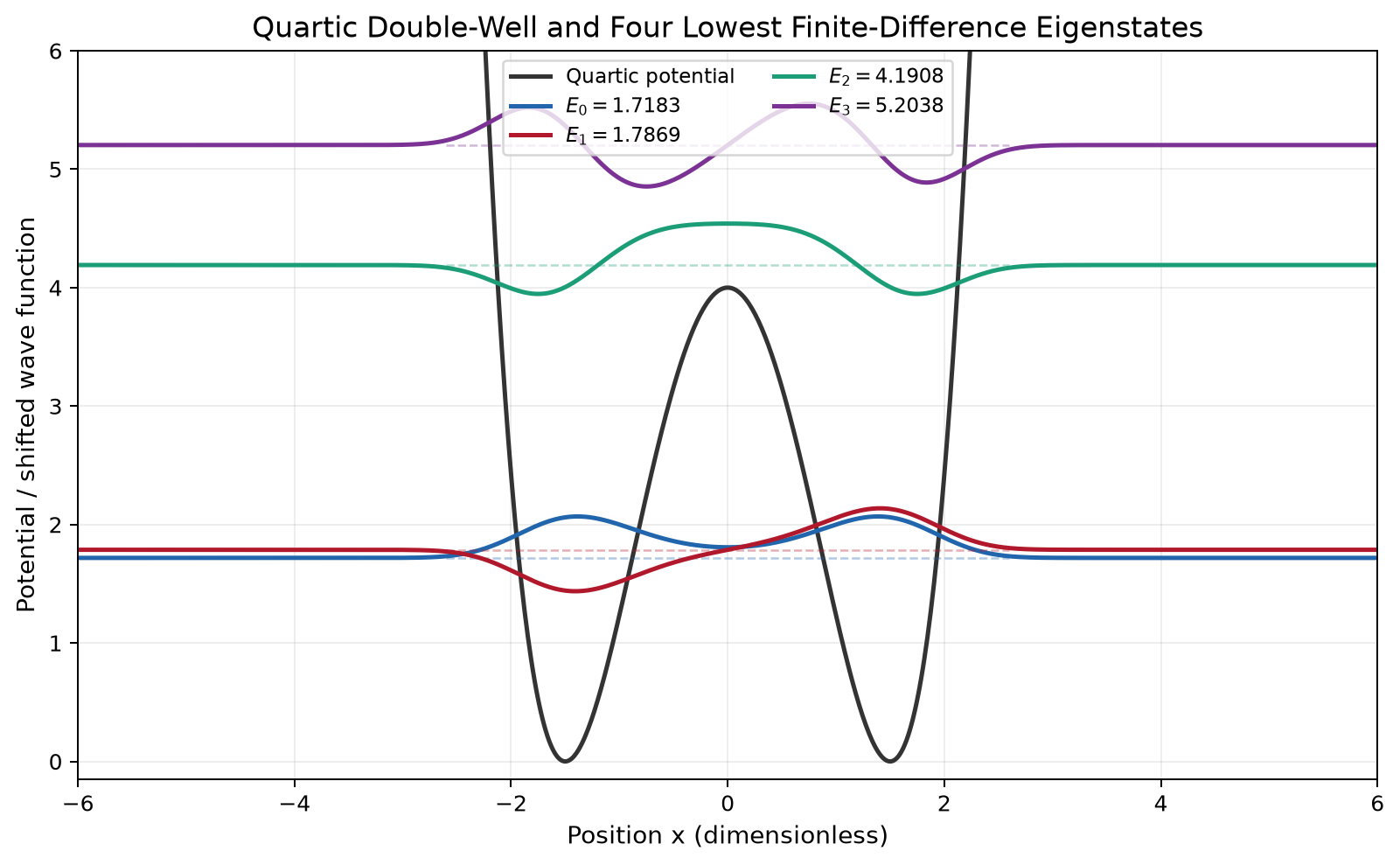
A symmetric double well, viewed at two levels of detail.
The dimensionless Hamiltonian is H = −d²/dy² + λ(y² − 1)² on −4 ≤ y ≤ 4. The scan varies the barrier parameter λ across nine values and the initial-state width s across seven values, producing 63 cases.
03 / Computational method
Separate model error from numerical error.
Each result passes through numerical-quality checks before entering the physical comparison.
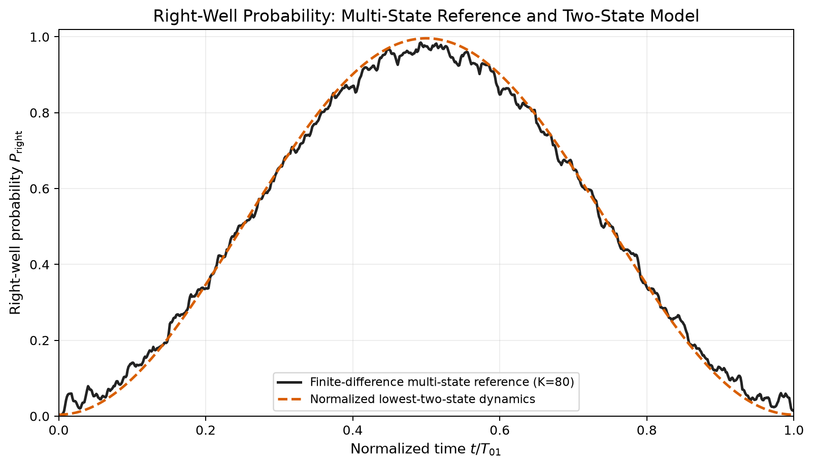
- 01Solve a finite-difference reference problem in continuous space and retain multiple eigenstates.
- 02Construct the lowest two-state approximation for the same potential and initial condition.
- 03Compare time-dependent observables across a controlled λ and s grid.
- 04Apply numerical-quality gates before interpreting an error metric as physically meaningful.
- Barrier parameter λ
- 2, 3, 4, 6, 8, 12, 18, 27, 40
- Initial width s
- 0.18 to 0.42
- Numerical audit
- K = 80, 120, 160, 240 eigenstates; focused grid checks at N = 801, 1201, 1601
 View full size (opens in a new tab)
04 / Key findings
Unresolved cases remain part of the result.
Numerical reliability depends on the metric being reported. All 63 cases pass the RMSE mask, while 52 pass the maximum-error and strict full-dynamics masks. The other 11 remain visible rather than being forced into a single reliable-or-failed label.
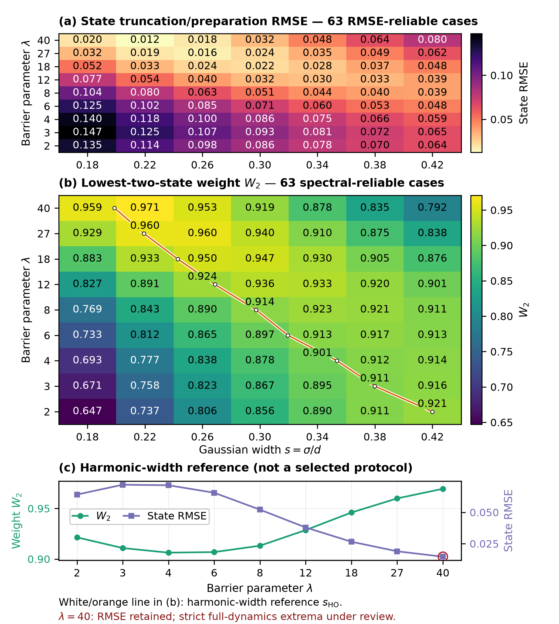
The strict-extrema review set contains four λ = 27 cases at s = 0.30, 0.34, 0.38, and 0.42, plus all seven λ = 40 cases. These cases still pass the RMSE, peak-time, and spectral masks; their review status is not evidence that the two-state physics failed. The λ = 40, s = 0.42 case also carries a separate maximum-error spatial-refinement review flag.
05 / Looking inside the error
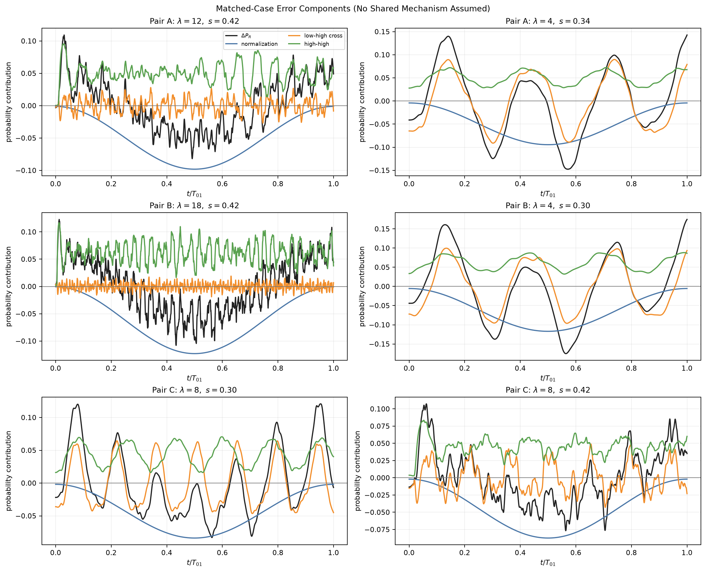
One similarity metric does not explain the whole difference.
Matched cases show that similar weight outside the lowest two states does not guarantee similar time-domain error.
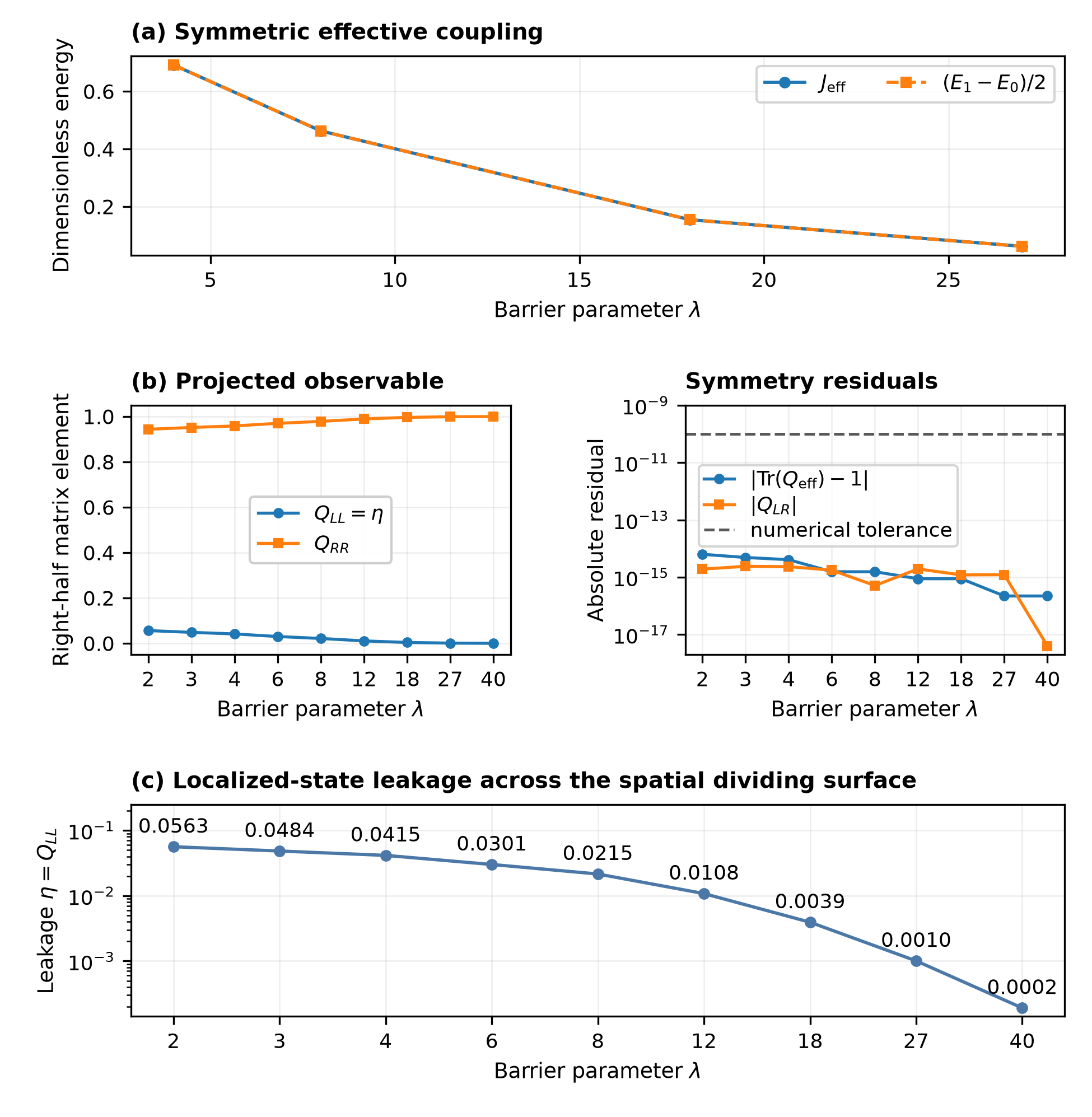
The separate 16-case mapping pilot contains four symmetric controls and twelve tilted cases. It is not an expansion of the 63-case symmetric preparation grid.
06 / Reproducibility
Regenerate, compare, and record.
At research snapshot 24186a9, 306 automated validation tests passed in an independent clean checkout (306 collected; 0 failed, 0 skipped, 0 xfailed, 0 xpassed). The full suite includes 285 previous tests and 21 added manuscript, figure, and integrity checks—not 21 new experiments. The reliability CSV and scientific generators are unchanged from the previous website snapshot, so the 63 / 52 / 11 counts remain unchanged. Figure 2 and Figure 5 use the updated manuscript versions.
Mentor-review manuscript draft v0.4. This is not a published or peer-reviewed paper, nor a student-approved final manuscript. Source-level layout checks passed; the v0.4 PDF layout still awaits manual Overleaf verification in this locked snapshot.
Locked commit: 24186a9908d00805b3720c97d67ed2eb1b7cb333
Official suite: .venv/bin/python -m pytest -q
07 / Limitations
What the current evidence does not yet establish.
Preserving these boundaries is part of the research method.
- 01
The reference is a finite-difference, multi-eigenstate numerical calculation—not an analytic exact solution.
- 02
A numerical-quality gate does not by itself define physical model validity.
- 03
No final physical-validity threshold has yet been selected.
- 04
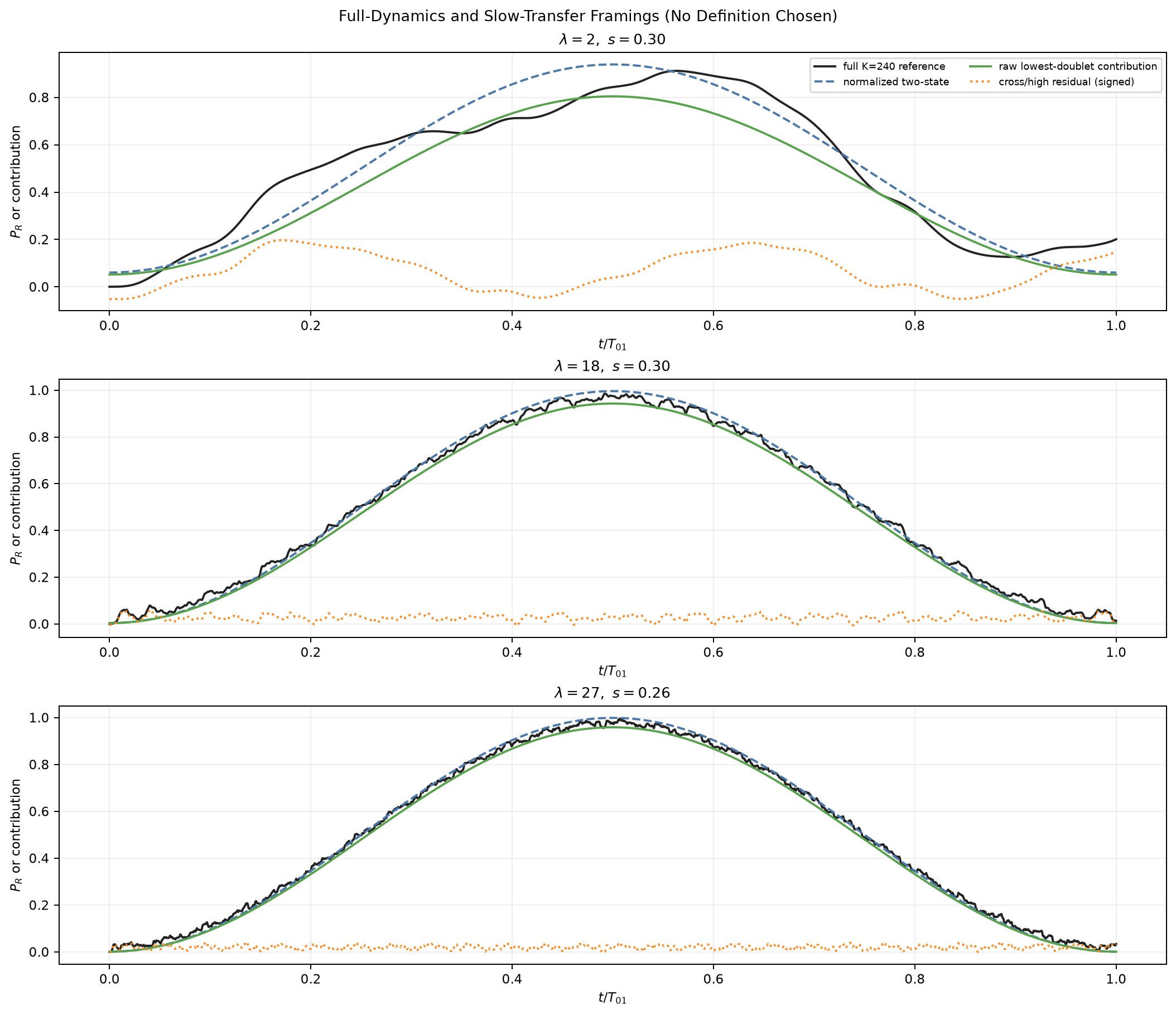
The project has not yet chosen whether the main target is full dynamics or the slow tunneling envelope.
- 05
Patterns observed on this finite grid should not be presented as universal causal laws.
08 / Current next steps
Define the physical claim before drawing the boundary.
Review the draft with a mentor, clarify whether full dynamics or a justified slow-tunneling observable best serves the question, and decide whether a physical accuracy criterion is needed.
Related Course Project
Qiskit, Trotterization, and a different source of error.
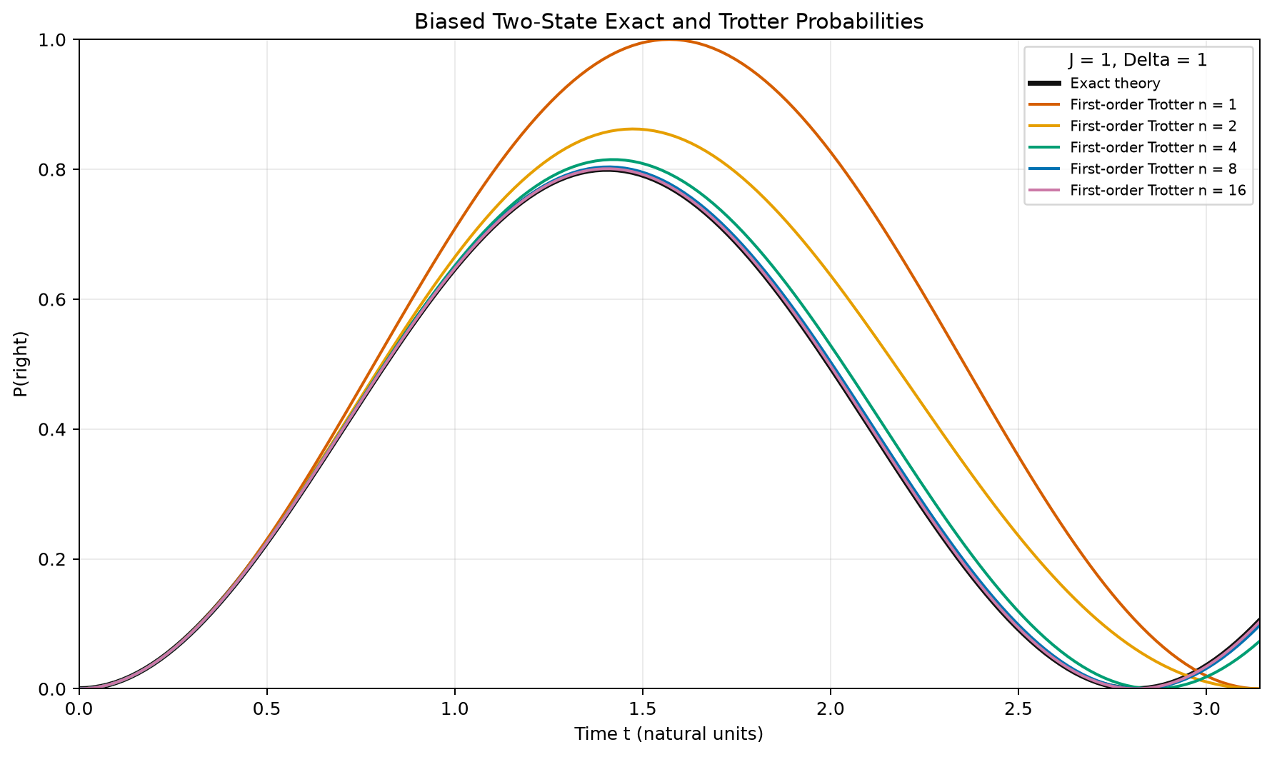
A Columbia Pre-College course project on Qiskit Trotterization later motivated this separate independent study. The course project examined digital-simulation error inside an effective two-state model; this later project studies model-reduction error by comparing that approximation with a continuous-space numerical reference.
 View full size (opens in a new tab)